El juego completo

Veamos un ejemplo completo. No hace falta entenderlo todo. Iremos viendo luego cada parte.

El ejemplo viene de aquí

Show the code

source(here::here("R/ggdag-mask.R"))
source(here::here("R/setup.R"))
library(tidyverse)
library(ggdag)
library(broom)

Pasos en el análisis causal.

Definir la pregunta causal
Especificar las asunciones, una forma es con un diagrama causal
Modelar las asunciones
Diagnosticar el modelo
Estimar el efecto causal
Análisis de sensibilidad

Datos

Show the code

library(dplyr)
library(ggplot2)
library(skimr)
library(broom)
library(halfmoon)

net_data <-  read.csv(here::here("data/net_data.csv"))

id: ID
net y net_num: Indican si se usa mosquitera (1) o no (0)
malaria_risk: Riesgo de malaria 0-100
income: ingresos, medida en dólares
health: Puntuación en salud de 0–100
household: Número de personas en el hogar
eligible: Indica si el hogar es eligible para programa de mosquitera gratis.
temperature: La temperatura media por las noches, en Celsius
resistance: Resistencia de los mosquitos locales al insecticida. Escala de 0–100, valores altos indican mayor resistencia

Show the code

skimr::skim(net_data |> select((-id)))

Data summary
Name	select(net_data, (-id))
Number of rows	1752
Number of columns	9
_______________________
Column type frequency:
logical	2
numeric	7
________________________
Group variables	None

Variable type: logical

skim_variable	n_missing	complete_rate	mean	count
net	0	1	0.26	FAL: 1298, TRU: 454
eligible	0	1	0.02	FAL: 1716, TRU: 36

Variable type: numeric

skim_variable	complete_rate	mean	sd	p0	p25	p50	p75	p100	hist
net_num	1	0.26	0.44	0.0	0.0	0.0	1.0	1.0	▇▁▁▁▃
malaria_risk	1	39.67	15.37	10.0	28.0	36.0	50.0	90.0	▃▇▅▂▁
income	1	897.76	191.24	330.0	764.8	893.0	1031.0	1484.0	▁▅▇▅▁
health	1	50.21	19.35	5.0	37.0	50.0	64.0	100.0	▂▆▇▅▁
household	1	2.97	1.41	1.0	2.0	3.0	4.0	9.0	▇▇▂▁▁
temperature	1	23.93	4.10	15.6	20.9	23.8	27.1	32.2	▃▇▇▇▃
insecticide_resistance	1	50.08	14.44	5.0	40.0	50.0	60.0	95.0	▁▅▇▃▁

Show the code

DT::datatable(net_data)

Esp## Especificar cuestión causal

¿El uso de la mosquitera reduce el riesgo de malaria?

Show the code

net_data |>
  ggplot(aes(malaria_risk, fill = net)) +
  geom_density(color = NA, alpha = .8)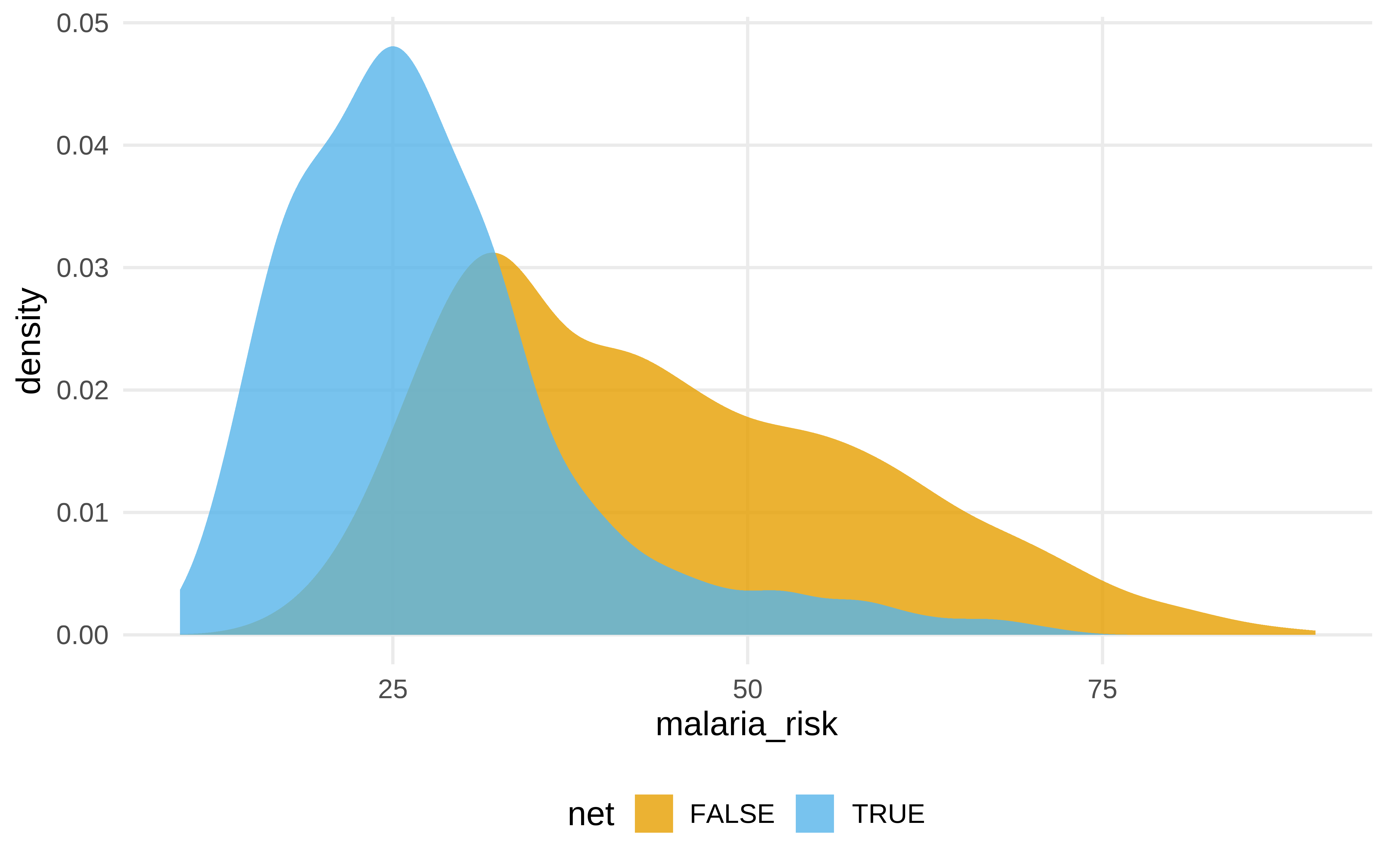

Show the code

net_data |>
  group_by(net) |>
  summarize(malaria_risk = mean(malaria_risk))

#> # A tibble: 2 × 2
#>   net   malaria_risk
#>   <lgl>        <dbl>
#> 1 FALSE         43.9
#> 2 TRUE          27.5

Show the code

# con una regresión obtenemos lo mismo
net_data |>
  lm(malaria_risk ~ net, data = _) |>
  tidy()

#> # A tibble: 2 × 5
#>   term        estimate std.error statistic  p.value
#>   <chr>          <dbl>     <dbl>     <dbl>    <dbl>
#> 1 (Intercept)     43.9     0.377     116.  0       
#> 2 netTRUE        -16.4     0.741     -22.1 1.10e-95

Show the code

net_data |>
  lm(malaria_risk ~  0 + net, data = _) |>
  tidy()

#> # A tibble: 2 × 5
#>   term     estimate std.error statistic   p.value
#>   <chr>       <dbl>     <dbl>     <dbl>     <dbl>
#> 1 netFALSE     43.9     0.377     116.  0        
#> 2 netTRUE      27.5     0.638      43.1 1.26e-277

Dibujar la asunciones

El uso de diagramas causales no es imprescindible, pero ayuda a explicitar las asunciones. Estas asunciones son nuestro modelo de como funcionar las relaciones entre las variables, pero puede que no sean correctas. Siempre habría que chequear el conocimiento experto y confrontar con otras explicaciones.

Show the code

library(tidyverse)
library(ggdag)
library(ggokabeito)
net_data <-  read_csv(here::here("data/net_data.csv"))
mosquito_dag <- dagify(
  malaria_risk ~ net + income + health + temperature + resistance,
  net ~ income + health + temperature + eligible + household,
  eligible ~ income + household,
  health ~ income,
  exposure = "net",
  outcome = "malaria_risk",
  coords = list(
    x = c(
      malaria_risk = 7,
      net = 3,
      income = 4,
      health = 5,
      temperature = 6,
      resistance = 8.5,
      eligible = 2,
      household = 1
    ),
    y = c(
      malaria_risk = 2,
      net = 2,
      income = 3,
      health = 1,
      temperature = 3,
      resistance = 2,
      eligible = 3,
      household = 2
    )
  ),
  labels = c(
    malaria_risk = "Risk of malaria",
    net = "Mosquito net",
    income = "Income",
    health = "Health",
    temperature = "Nighttime temperatures",
    resistance = "Insecticide resistance",
    eligible = "Eligible for program",
    household = "Number in the household"
  )
)

p1 <- mosquito_dag |>
  tidy_dagitty() |>
  node_status() |>
  ggplot(
    aes(x, y, xend = xend, yend = yend, color = status)
  ) +
  geom_dag_edges() +
  geom_dag_point() +
  geom_dag_label(color = "black") +
  # geom_dag_label_repel() +
  scale_color_okabe_ito(na.value = "grey90") +
  theme_dag() +
  theme(legend.position = "none") +
  coord_cartesian(clip = "off")
p1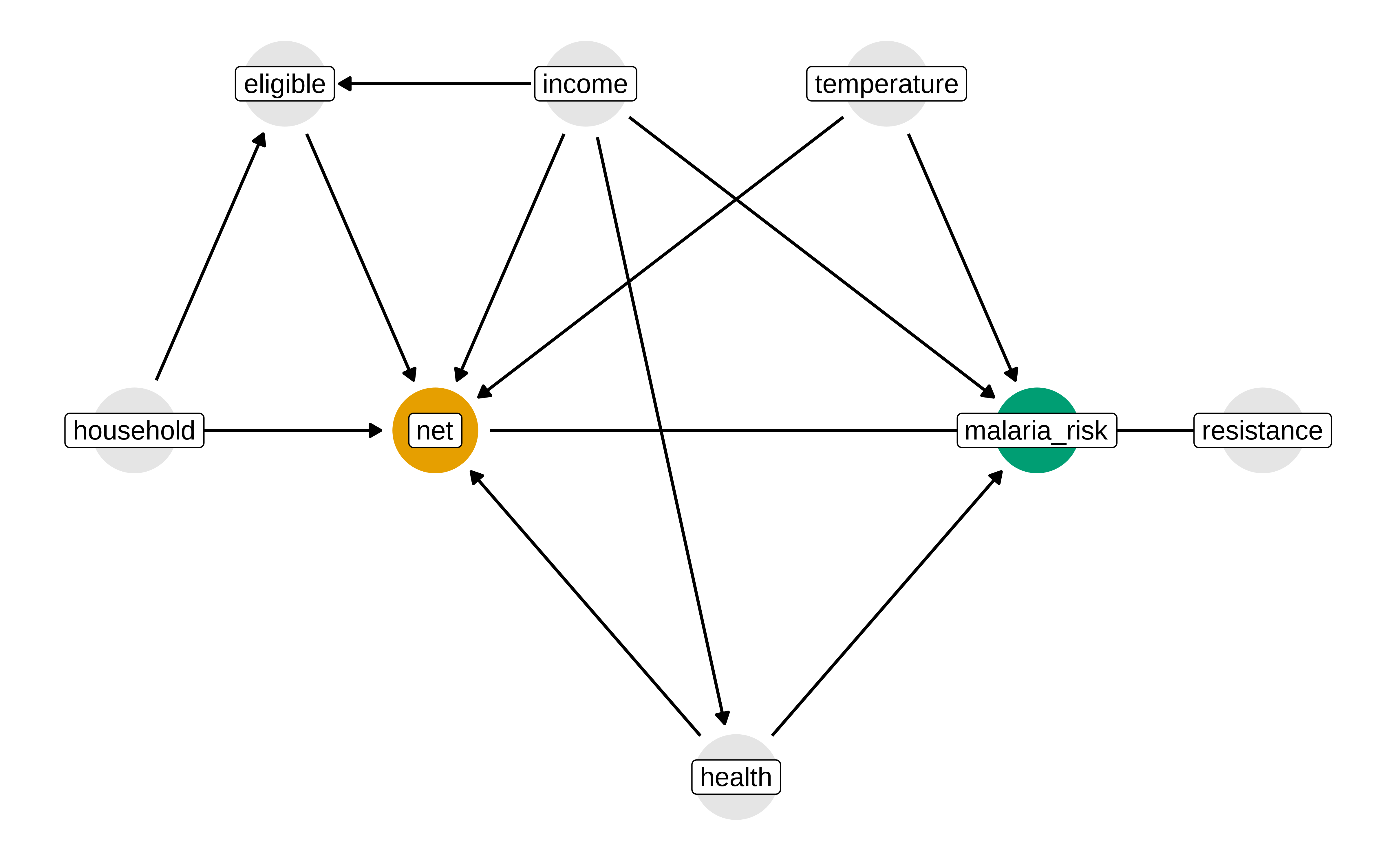

Modelar las asunciones

Dado el DAG anterior, vamos a utilizar una técnica conocida como propensity score weighting. El objetivo de esta técnica es crear una pseudopoblación que imite como habrían sido los datos si se hubiera hecho un RCT (Randomized Controlled Trial).

Show the code

propensity_model <- glm(
  net ~ income + health + temperature,
  data = net_data,
  family = binomial()
)

Show the code

head(predict(propensity_model, type = "response"))

#>      1      2      3      4      5      6 
#> 0.2464 0.2178 0.3230 0.2307 0.2789 0.3060

Show the code

net_data_with_ipw <- net_data |>
  mutate(
    propensity_score = predict(propensity_model, type = "response")
  ) |>
  mutate(
    ipw = ifelse(net_num == 1, 1 / propensity_score, 1 / (1 - propensity_score))
  )

Vemos los ipw. Si una observación ha caído en control pero tiene una probabilidad en el modelo de propensity score de 0.9, su peso es de 1 /(1-0.9) = 10 . Es decir, este individuo se considera un muy buen contrafactual para un individuo de iguales características que hubiera caido en tratamiento.

Show the code

net_data_with_ipw |>
  filter(net_num == 0) |>
  select(net,net_num, propensity_score, ipw) |>
  arrange(desc(propensity_score)) |>
  head()

#> # A tibble: 6 × 4
#>   net   net_num propensity_score   ipw
#>   <lgl>   <dbl>            <dbl> <dbl>
#> 1 FALSE       0            0.475  1.90
#> 2 FALSE       0            0.468  1.88
#> 3 FALSE       0            0.461  1.86
#> 4 FALSE       0            0.451  1.82
#> 5 FALSE       0            0.447  1.81
#> 6 FALSE       0            0.438  1.78

Show the code

net_data_with_ipw |>
  filter(net_num ==1) |>
  arrange(propensity_score) |>
  select(net,net_num, propensity_score, ipw) |>
  head()

#> # A tibble: 6 × 4
#>   net   net_num propensity_score   ipw
#>   <lgl>   <dbl>            <dbl> <dbl>
#> 1 TRUE        1            0.117  8.56
#> 2 TRUE        1            0.120  8.33
#> 3 TRUE        1            0.126  7.92
#> 4 TRUE        1            0.136  7.36
#> 5 TRUE        1            0.138  7.27
#> 6 TRUE        1            0.139  7.19

Diagnosticar las asunciones

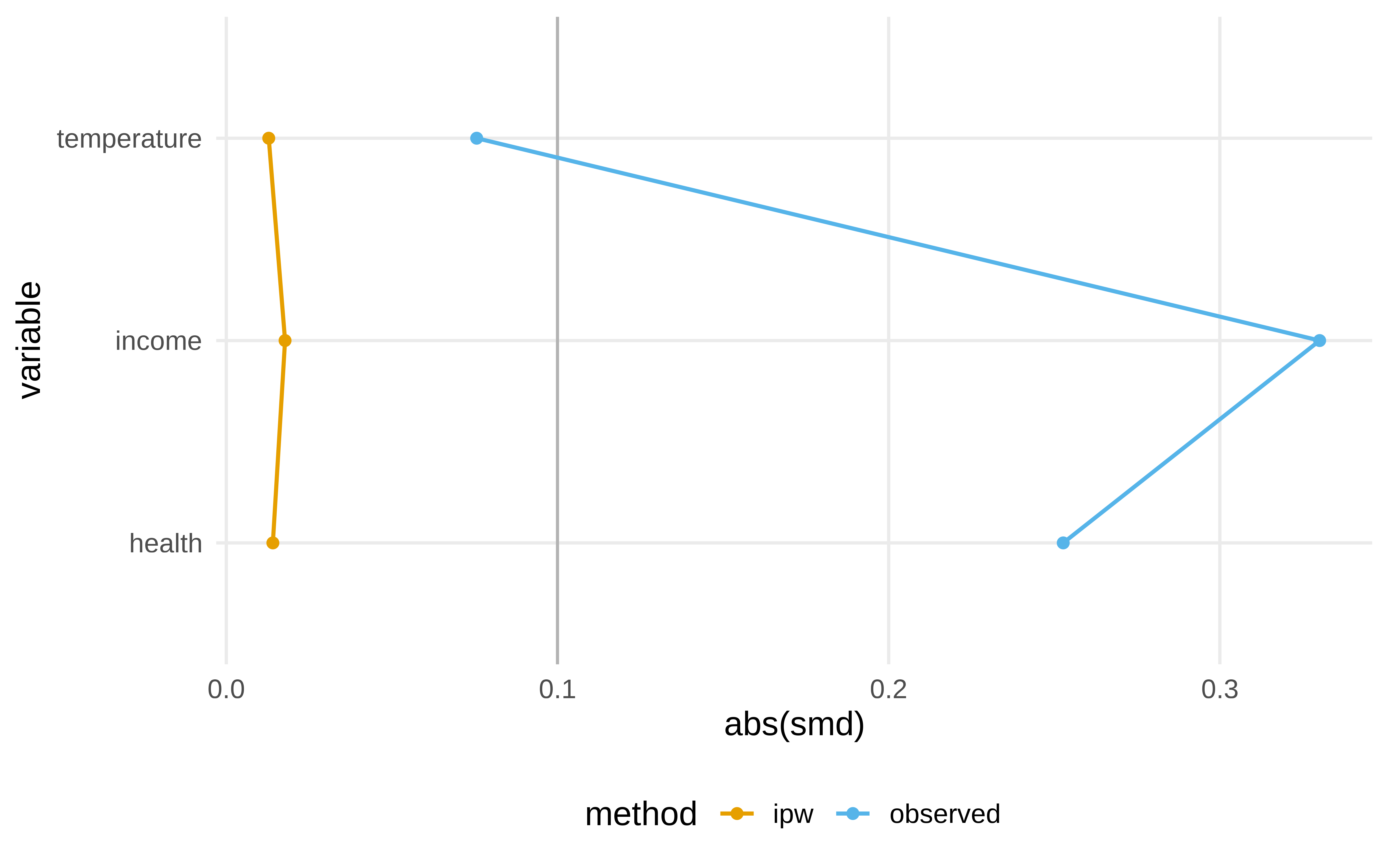
¿Qué es lo que ha cambiado al hacer el ipw?

Show the code

library(halfmoon)

net_data_with_ipw |> 
  ggplot( aes(propensity_score)) +
  geom_mirror_histogram(
    aes(fill = net),
    bins = 50
  ) +
  scale_y_continuous(labels = abs) +
  labs(x = "propensity score")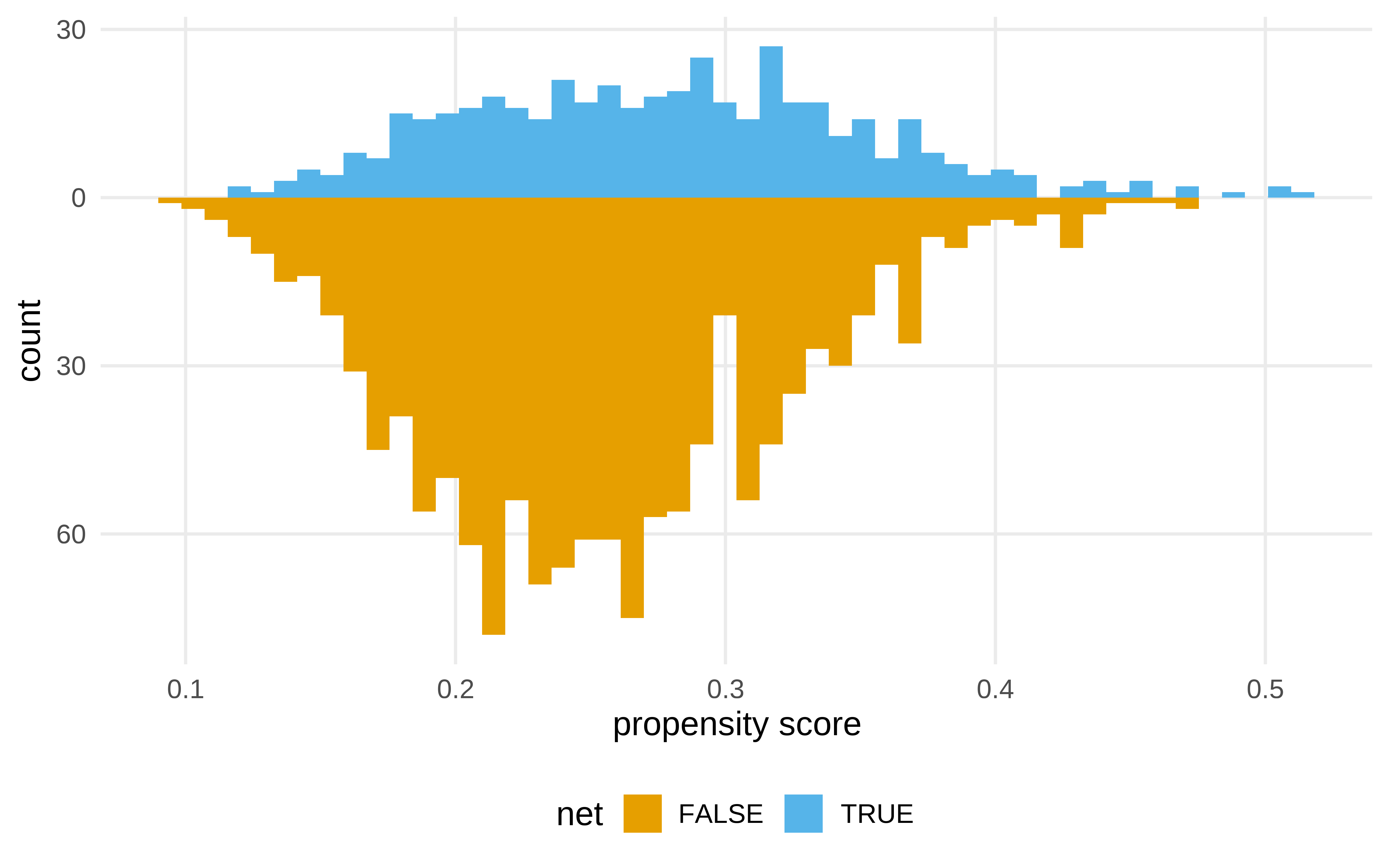

Show the code

plot_df <- tidy_smd(
  net_data_with_ipw,
  c(income, health, temperature),
  .group = net,
  .wts = ipw
)

ggplot(
  plot_df,
  aes(
    x = abs(smd),
    y = variable,
    group = method,
    color = method
  )
) +
  geom_love()

Estimar el efecto causal

Usando ipw

Show the code

net_data_with_ipw |>
  lm(malaria_risk ~  net, data = _, weights = ipw) |>
  tidy(conf.int = TRUE) |>
  filter(term == "netTRUE")

#> # A tibble: 1 × 7
#>   term   estimate std.error statistic  p.value conf.low
#>   <chr>     <dbl>     <dbl>     <dbl>    <dbl>    <dbl>
#> 1 netTR…    -12.5     0.624     -20.1 5.50e-81    -13.8
#> # ℹ 1 more variable: conf.high <dbl>

Pero una vez se ha hecho el ipw, la varianza del estimador que da el modelo lm no es correcta, hay que calcularla usando otras técnicas, como estimadores robustos o bootstrap. Usaremos bootstrap

Show the code

library(rsample)

# todo el proceso
fit_ipw <- function(split, ...) {
  # get bootstrapped data sample with `rsample::analysis()`
  .df <- analysis(split)

  # fit propensity score model
  propensity_model <- glm(
    net ~ income + health + temperature,
    data = .df,
    family = binomial()
  )

  # calculate inverse probability weights
  .df <-  .df |>
  mutate(
    propensity_score = predict(propensity_model, type = "response")
  ) |>
  mutate(
    ipw = ifelse(net_num == 1, 1 / propensity_score, 1 / (1 - propensity_score))
  )


  # fit correctly bootstrapped ipw model
  lm(malaria_risk ~ net, data = .df, weights = ipw) |>
    tidy()
}

Show the code

bootstrapped_net_data <- bootstraps(
  net_data,
  times = 1000,
  # required to calculate CIs later
  apparent = TRUE
)

bootstrapped_net_data

#> # Bootstrap sampling with apparent sample 
#> # A tibble: 1,001 × 2
#>    splits             id           
#>    <list>             <chr>        
#>  1 <split [1752/633]> Bootstrap0001
#>  2 <split [1752/633]> Bootstrap0002
#>  3 <split [1752/639]> Bootstrap0003
#>  4 <split [1752/640]> Bootstrap0004
#>  5 <split [1752/648]> Bootstrap0005
#>  6 <split [1752/641]> Bootstrap0006
#>  7 <split [1752/669]> Bootstrap0007
#>  8 <split [1752/647]> Bootstrap0008
#>  9 <split [1752/619]> Bootstrap0009
#> 10 <split [1752/661]> Bootstrap0010
#> # ℹ 991 more rows

Show the code

# En cada muestra ejecutamos el proceso completo

ipw_results <- bootstrapped_net_data |>
  mutate(boot_fits = map(splits, fit_ipw))

ipw_results

#> # Bootstrap sampling with apparent sample 
#> # A tibble: 1,001 × 3
#>    splits             id            boot_fits       
#>    <list>             <chr>         <list>          
#>  1 <split [1752/633]> Bootstrap0001 <tibble [2 × 5]>
#>  2 <split [1752/633]> Bootstrap0002 <tibble [2 × 5]>
#>  3 <split [1752/639]> Bootstrap0003 <tibble [2 × 5]>
#>  4 <split [1752/640]> Bootstrap0004 <tibble [2 × 5]>
#>  5 <split [1752/648]> Bootstrap0005 <tibble [2 × 5]>
#>  6 <split [1752/641]> Bootstrap0006 <tibble [2 × 5]>
#>  7 <split [1752/669]> Bootstrap0007 <tibble [2 × 5]>
#>  8 <split [1752/647]> Bootstrap0008 <tibble [2 × 5]>
#>  9 <split [1752/619]> Bootstrap0009 <tibble [2 × 5]>
#> 10 <split [1752/661]> Bootstrap0010 <tibble [2 × 5]>
#> # ℹ 991 more rows

Show the code

ipw_results$boot_fits[[1]]

#> # A tibble: 2 × 5
#>   term        estimate std.error statistic  p.value
#>   <chr>          <dbl>     <dbl>     <dbl>    <dbl>
#> 1 (Intercept)     42.9     0.445      96.4 0       
#> 2 netTRUE        -13.0     0.630     -20.6 1.03e-84

Show the code

# pintamos los resultados

Show the code

ipw_results |>
  mutate(
    estimate = map_dbl(
      boot_fits,
      # pull the `estimate` for `netTRUE` for each fit
      # \(.fit) .fit |>
        function(x) {
          x |>
        filter(term == "netTRUE") |>
        pull(estimate)
          }
    )
  ) |>
  ggplot(aes(estimate)) +
  geom_histogram(fill = "#D55E00FF", color = "white", alpha = 0.8)

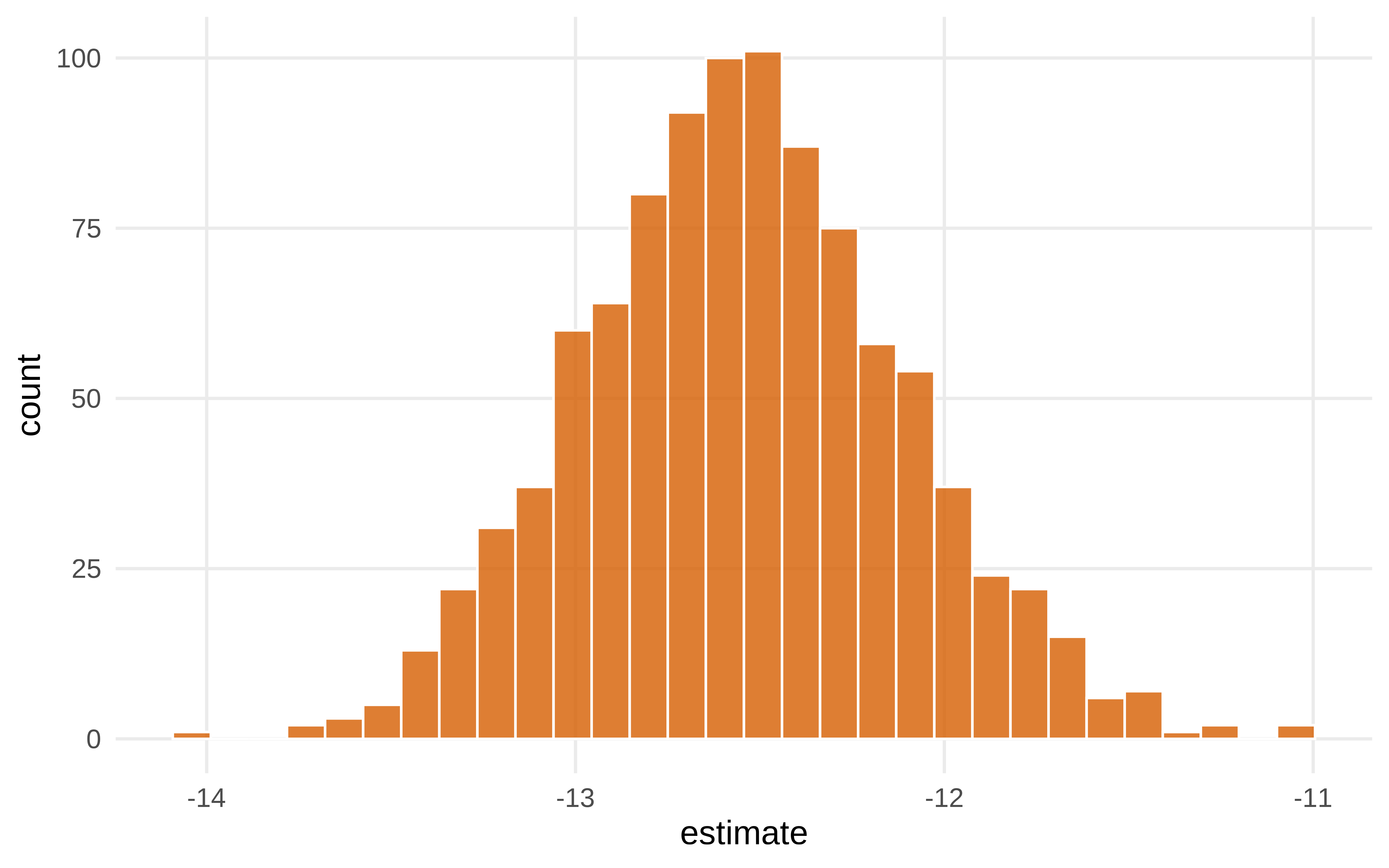
Show the code

boot_estimate <- ipw_results |>
  # intervalo usando percentil
  int_pctl(boot_fits, alpha = 0.01) |>
  filter(term == "netTRUE")

boot_estimate

#> # A tibble: 1 × 6
#>   term    .lower .estimate .upper .alpha .method   
#>   <chr>    <dbl>     <dbl>  <dbl>  <dbl> <chr>     
#> 1 netTRUE  -13.6     -12.5  -11.4   0.01 percentile

Usando reglas de Pearl

Pensemos como cortar los caminos no causales

Show the code

p1

Pero la librería dagitty nos sirve para esto

Show the code

dagitty::adjustmentSets(mosquito_dag, effect = "total")

#> { health, income, temperature }

Show the code

ggdag_adjustment_set(mosquito_dag, effect = "total")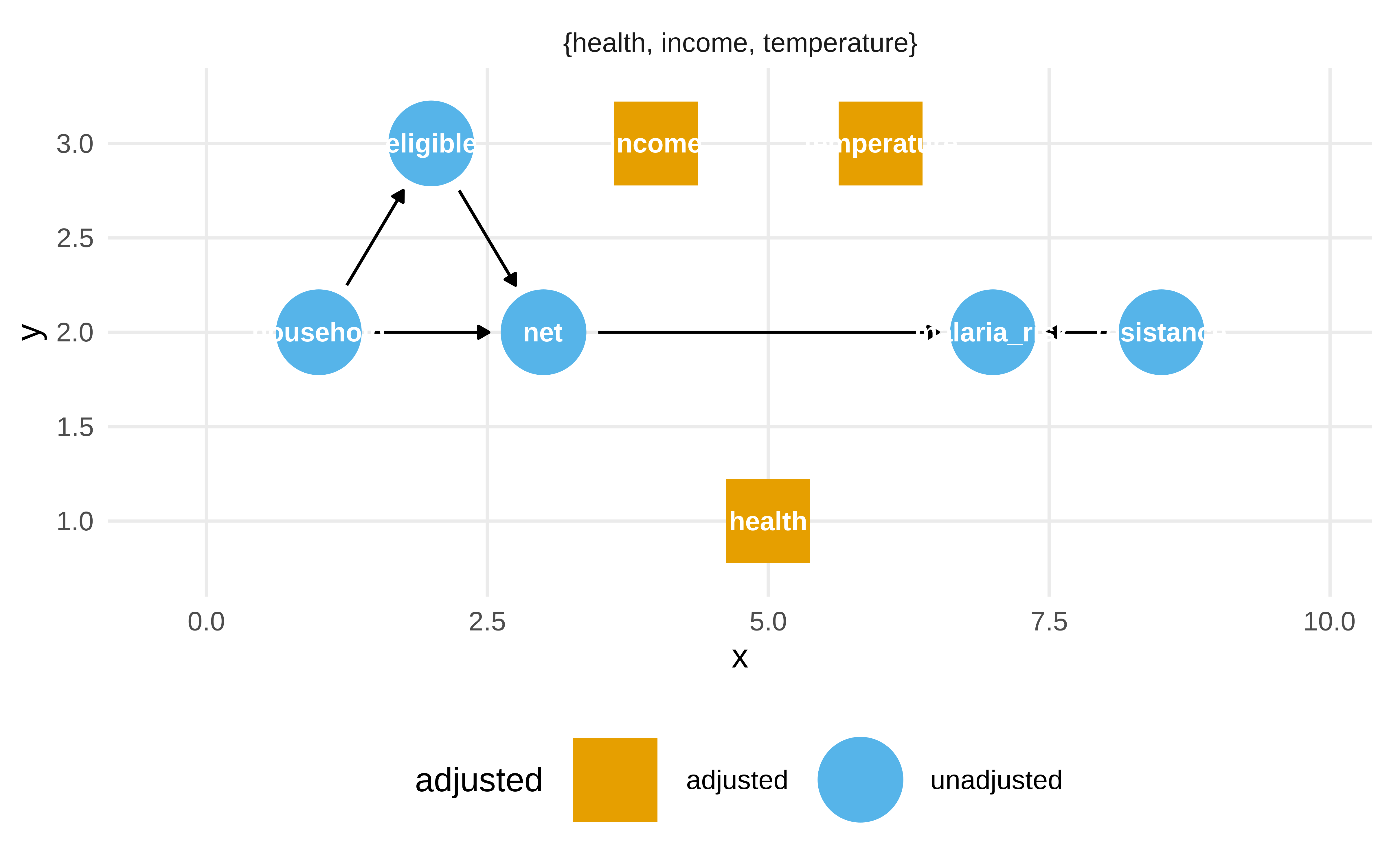

Show the code

lm(malaria_risk ~ net + income + temperature + health, data = net_data) |>
  tidy(conf.int = TRUE) |>
  filter(term == "netTRUE")

#> # A tibble: 1 × 7
#>   term  estimate std.error statistic   p.value conf.low
#>   <chr>    <dbl>     <dbl>     <dbl>     <dbl>    <dbl>
#> 1 netT…    -12.0     0.314     -38.2 2.69e-232    -12.6
#> # ℹ 1 more variable: conf.high <dbl>

Show the code

net_data |>
  ggplot(aes(income, fill = net)) +
  geom_density(color = NA, alpha = .8)

Show the code

net_data |>
  ggplot(aes(temperature, fill = net)) +
  geom_density(color = NA, alpha = .8)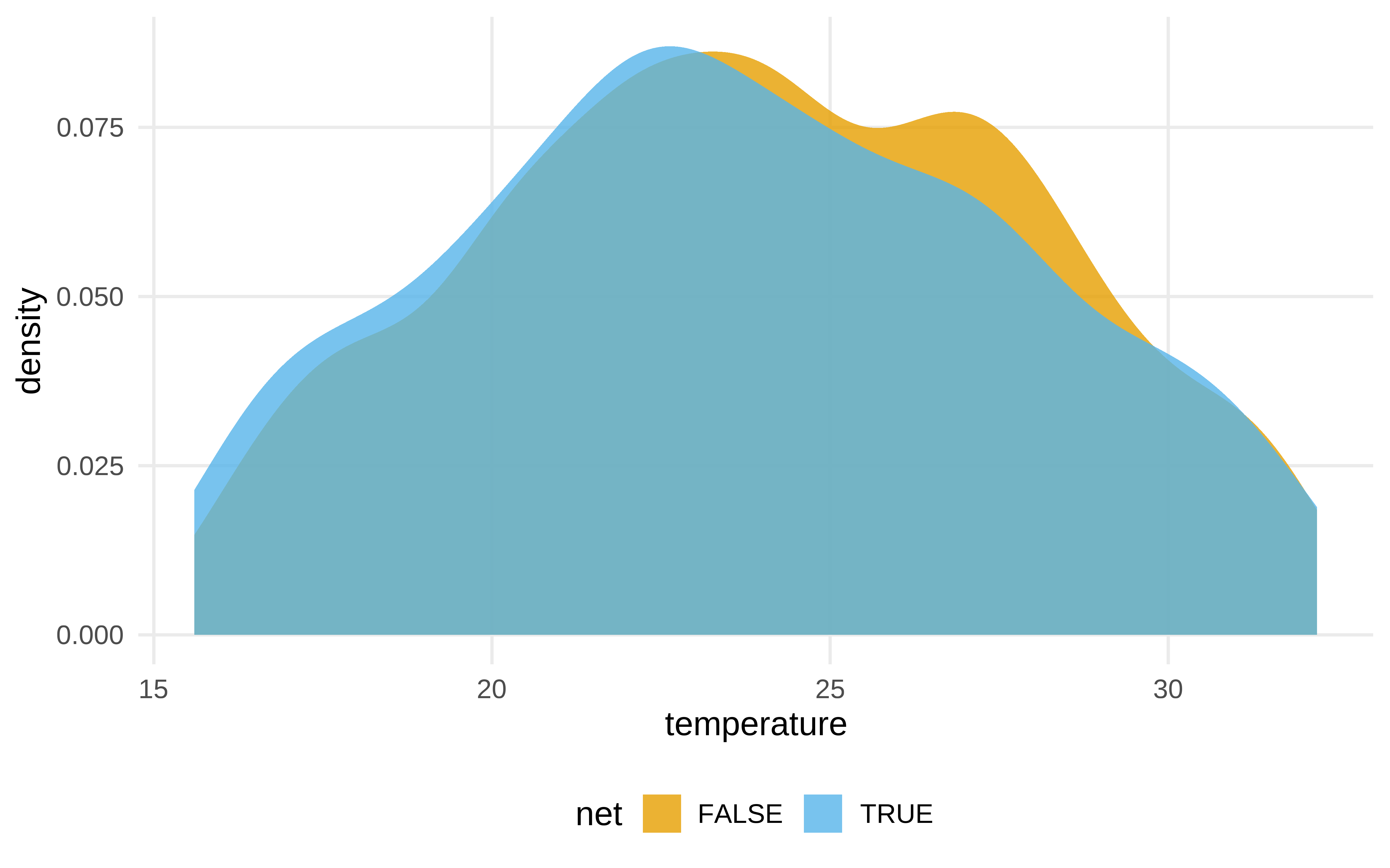

Show the code

net_data |>
  ggplot(aes(health , fill = net)) +
  geom_density(color = NA, alpha = .8)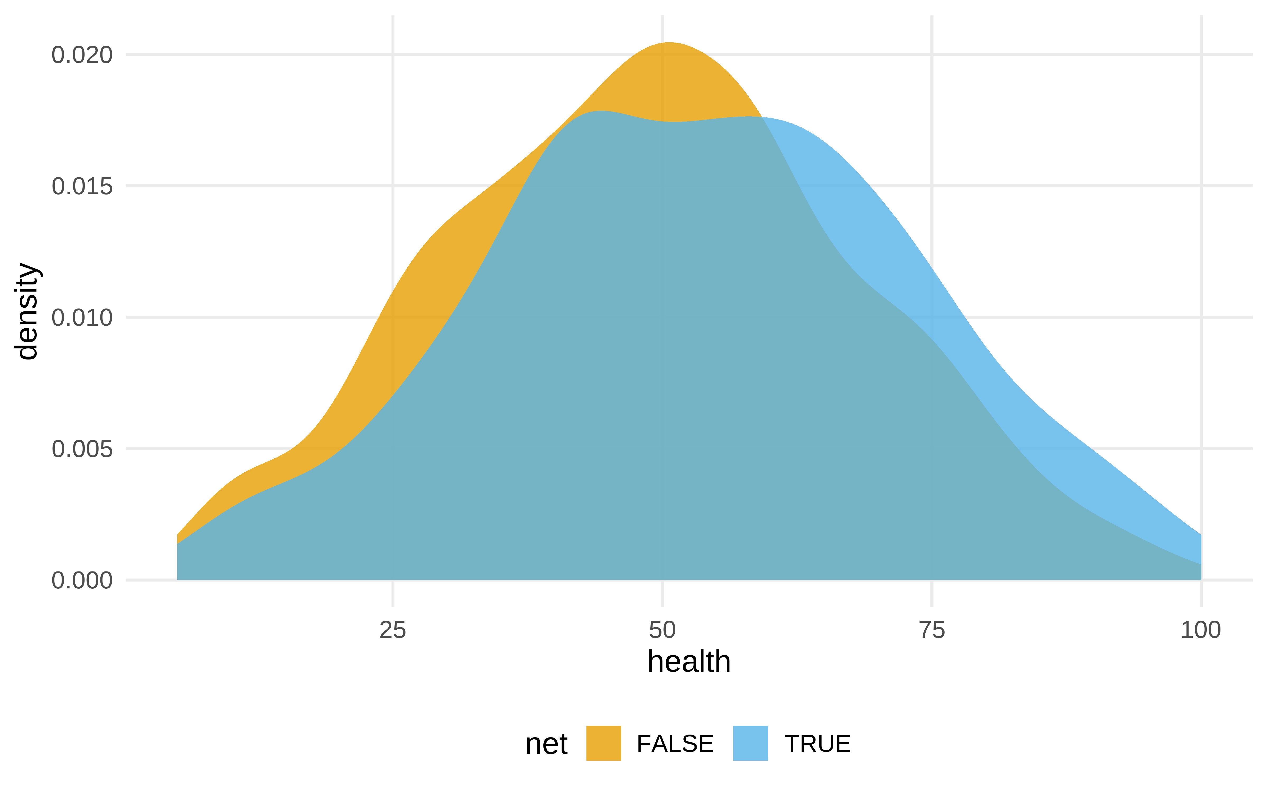

Modelo bayesiano

Show the code

library(cmdstanr)
library(brms)
library(posterior) # para cosas como rvar

options(brms.backend = "cmdstanr")

Show the code

m_bayesian <- brm(
  malaria_risk ~ net + income + temperature + health ,
  data = net_data,
  seed = 48,
  chains = 4,
  iter = 4000,
  warmup = 1000,
  cores = 4, 
  file = here::here("brms_stan_models/net_1"),
  file_refit = "on_change"
  
)

# hqy que evitar el exceso de decimales dando impresión de falsa exactitud
m_bayesian

#>  Family: gaussian 
#>   Links: mu = identity; sigma = identity 
#> Formula: malaria_risk ~ net + income + temperature + health 
#>    Data: net_data (Number of observations: 1752) 
#>   Draws: 4 chains, each with iter = 4000; warmup = 1000; thin = 1;
#>          total post-warmup draws = 12000
#> 
#> Regression Coefficients:
#>             Estimate Est.Error l-95% CI u-95% CI Rhat
#> Intercept      79.36      1.03    77.35    81.39 1.00
#> netTRUE       -12.00      0.31   -12.61   -11.39 1.00
#> income         -0.08      0.00    -0.08    -0.07 1.00
#> temperature     1.01      0.03     0.94     1.08 1.00
#> health          0.14      0.01     0.12     0.16 1.00
#>             Bulk_ESS Tail_ESS
#> Intercept      11125    10282
#> netTRUE        10925     8382
#> income         11593     9652
#> temperature    10913     8132
#> health         11001     9015
#> 
#> Further Distributional Parameters:
#>       Estimate Est.Error l-95% CI u-95% CI Rhat
#> sigma     5.70      0.10     5.51     5.89 1.00
#>       Bulk_ESS Tail_ESS
#> sigma    12498     8777
#> 
#> Draws were sampled using sample(hmc). For each parameter, Bulk_ESS
#> and Tail_ESS are effective sample size measures, and Rhat is the potential
#> scale reduction factor on split chains (at convergence, Rhat = 1).

Show the code

round(posterior_summary(m_bayesian, variable = "b_netTRUE"), 2)

#>           Estimate Est.Error   Q2.5  Q97.5
#> b_netTRUE      -12      0.31 -12.61 -11.39

Show the code

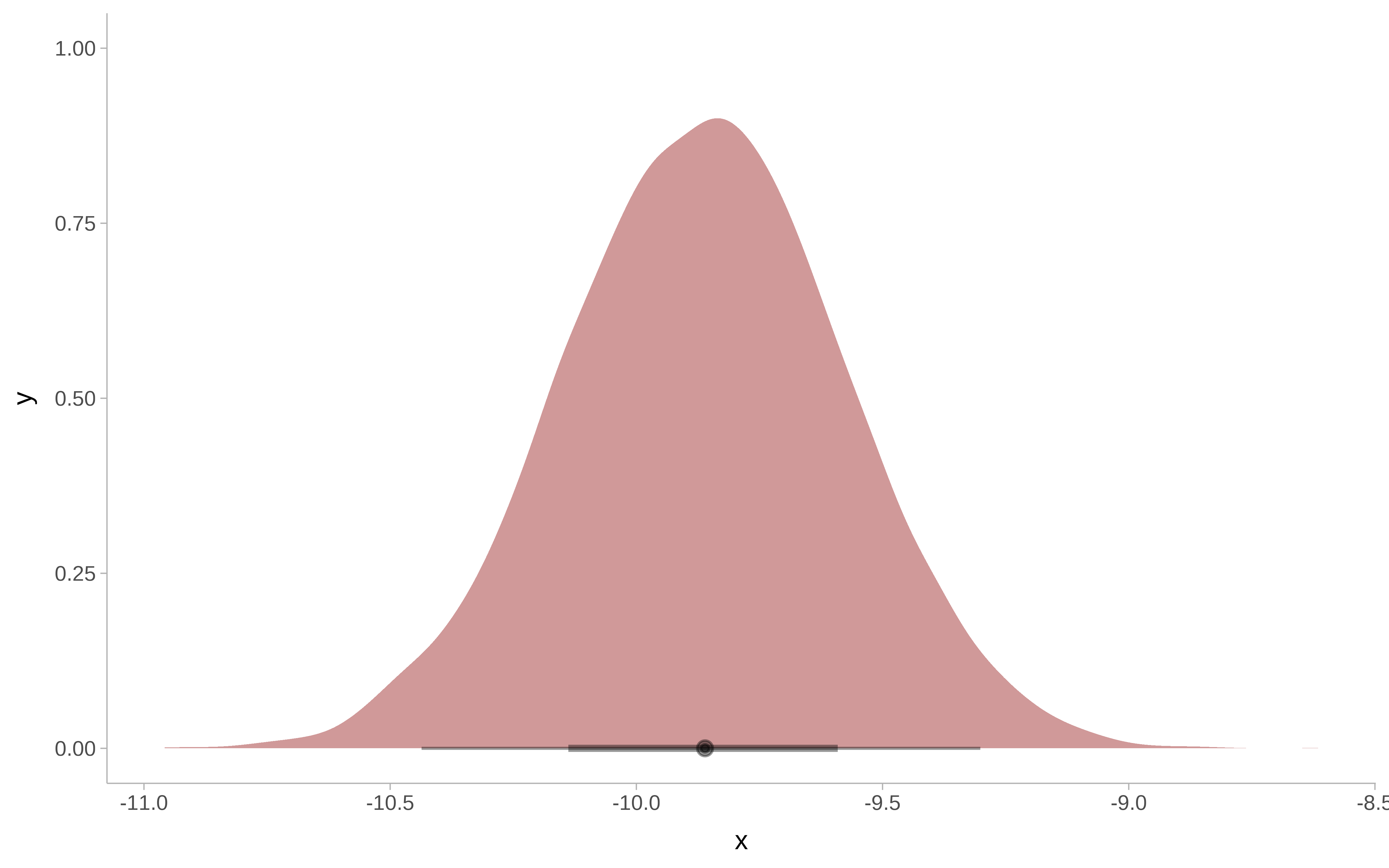
m_bayesian |>
  as_tibble() |>
  ggplot() +
  ggdist::stat_halfeye(
    aes( x = b_netTRUE),
    fill = "darkred",
    alpha = 0.4)  +
  ggdist::theme_ggdist()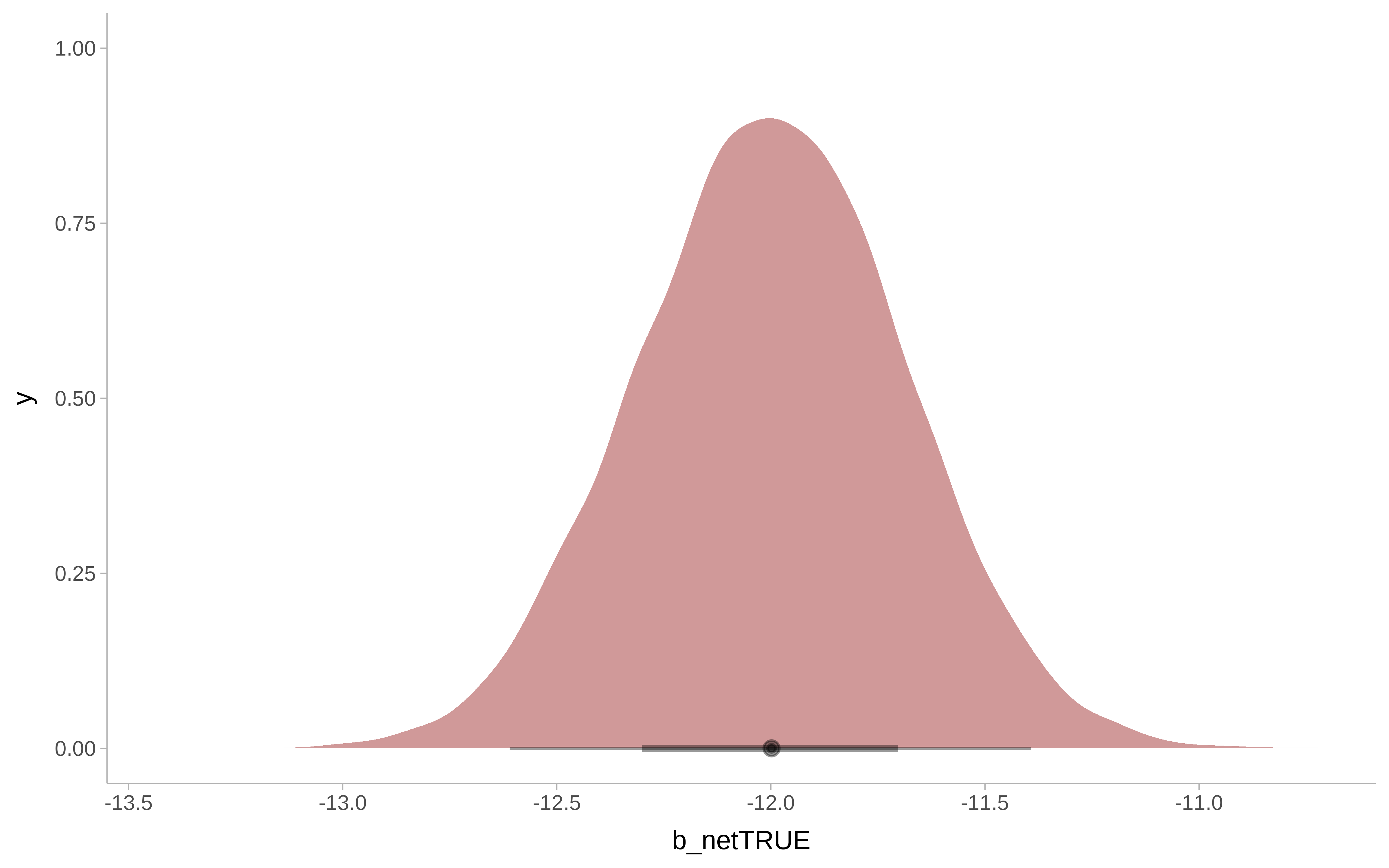

Análisis de sensibilidad

Y si hubiera una variable de confusión no observada?. Si fuera un RCT, el mismo mecanismo de aleatorización nos protege frente a esas variables, pero no en un estudio observacional.

Imaginemos que existe una variable de confusión que es resistencia genética de la población a la malaria.

Suponemos lo siguiente.

Está asociada con la variable respuesta, porque en media la gente con resistencia genética tiene una reducción de riesgo alrededor de 10.
Está asociada con la variable de tratamiento, puesto que entre los que usan mosquiteras, el 26 % tienen esta resistencia. Pero entre los que no usan mosquiteras, solo el 5% la tienen.

Con la librería tipr se puede inferir cuál sería el efecto si existiera ese confounder no observado.

Verdadero DAG

Y después de todo, como los datos son simulados sabemos que existe una variable de confusión

Show the code

mosquito_dag_full <- dagify(
  malaria_risk ~ net + income + health + temperature + insecticide_resistance + genetic_resistance,
  net ~ income + health + temperature + eligible + household + genetic_resistance,
  eligible ~ income + household,
  health ~ income,
  exposure = "net",
  outcome = "malaria_risk",
  coords = list(
    x = c(
      malaria_risk = 7,
      net = 3,
      income = 4,
      health = 5,
      temperature = 6,
      insecticide_resistance = 8.5,
      eligible = 2,
      household = 1,
      genetic_resistance = 8.5
    ),
    y = c(
      malaria_risk = 2,
      net = 2,
      income = 3,
      health = 1,
      temperature = 3,
      insecticide_resistance = 2,
      eligible = 3,
      household = 2,
      genetic_resistance = 1
    )
  ),
  labels = c(
    malaria_risk = "Risk of malaria",
    net = "Mosquito net",
    income = "Income",
    health = "Health",
    temperature = "Nighttime temperatures",
    insecticide_resistance = "Insecticide resistance",
    eligible = "Eligible for program",
    household = "Number in household",
    genetic_resistance = "Malaria resistance"
  )
)

mosquito_dag_full |>
  tidy_dagitty() |>
  node_status() |>
  ggplot(
    aes(x, y, xend = xend, yend = yend, color = status)
  ) +
  geom_dag_edges() +
  geom_dag_point() +
  geom_dag_label_repel() +
  scale_color_okabe_ito(na.value = "grey90") +
  theme_dag() +
  theme(legend.position = "none") +
  coord_cartesian(clip = "off")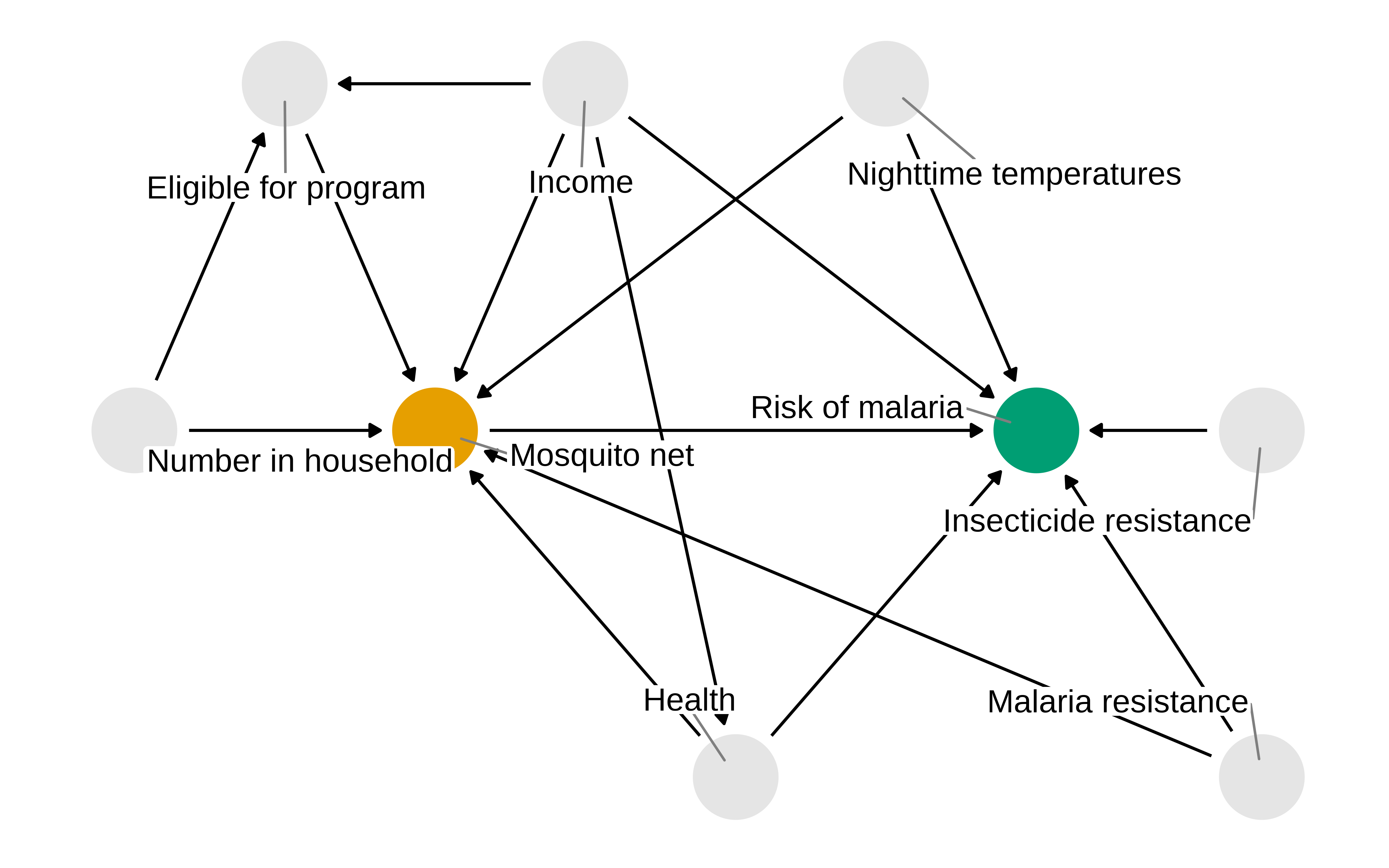

Show the code

net_data_full <- read.csv(here::here("data/net_data_full.csv"))
glimpse(net_data_full)

#> Rows: 1,752
#> Columns: 11
#> $ id                     <int> 1, 2, 3, 4, 5, 6, 7, 8…
#> $ net                    <lgl> FALSE, FALSE, FALSE, F…
#> $ net_num                <int> 0, 0, 0, 0, 0, 0, 0, 0…
#> $ malaria_risk           <int> 38, 48, 32, 55, 36, 30…
#> $ income                 <int> 779, 700, 1083, 753, 9…
#> $ health                 <int> 35, 35, 58, 68, 46, 37…
#> $ household              <int> 1, 3, 3, 3, 5, 3, 1, 2…
#> $ eligible               <lgl> FALSE, FALSE, FALSE, F…
#> $ temperature            <dbl> 18.3, 18.6, 24.2, 19.1…
#> $ insecticide_resistance <int> 38, 40, 70, 57, 59, 49…
#> $ genetic_resistance     <int> 0, 0, 0, 0, 0, 0, 0, 1…

Show the code

fit_ipw_full <- function(split, ...) {
  # get bootstrapped data sample with `rsample::analysis()`
  .df <- analysis(split)

  # fit propensity score model
  propensity_model <- glm(
    net ~ income + health + temperature + genetic_resistance,,
    data = .df,
    family = binomial()
  )

  # calculate inverse probability weights
  .df <-  .df |>
  mutate(
    propensity_score = predict(propensity_model, type = "response")
  ) |>
  mutate(
    ipw = ifelse(net_num == 1, 1 / propensity_score, 1 / (1 - propensity_score))
  )


  # fit correctly bootstrapped ipw model
  lm(malaria_risk ~ net, data = .df, weights = ipw) |>
    tidy()
}

Show the code

bootstrapped_net_data_full <- bootstraps(
  net_data_full,
  times = 1000,
  # required to calculate CIs later
  apparent = TRUE
)

ipw_results_full <- bootstrapped_net_data_full |>
  mutate(boot_fits = map(splits, fit_ipw_full))

boot_estimate_full <- ipw_results_full |>
  # calculate T-statistic-based CIs
  int_t(boot_fits) |>
  filter(term == "netTRUE")

boot_estimate_full

#> # A tibble: 1 × 6
#>   term    .lower .estimate .upper .alpha .method  
#>   <chr>    <dbl>     <dbl>  <dbl>  <dbl> <chr>    
#> 1 netTRUE  -11.3     -10.2  -9.34   0.05 student-t

Show the code

m_bayesian_full <- brm(
  malaria_risk ~ net + income + temperature + health + genetic_resistance ,
  data = net_data_full,
  seed = 48,
  chains = 4,
  iter = 4000,
  warmup = 1000,
  cores = 4, 
  file = here::here("brms_stan_models/net_2"),
  file_refit = "on_change"
  
)

summary(m_bayesian_full)

#>  Family: gaussian 
#>   Links: mu = identity; sigma = identity 
#> Formula: malaria_risk ~ net + income + temperature + health + genetic_resistance 
#>    Data: net_data_full (Number of observations: 1752) 
#>   Draws: 4 chains, each with iter = 4000; warmup = 1000; thin = 1;
#>          total post-warmup draws = 12000
#> 
#> Regression Coefficients:
#>                    Estimate Est.Error l-95% CI
#> Intercept             79.29      0.90    77.52
#> netTRUE               -9.86      0.29   -10.44
#> income                -0.08      0.00    -0.08
#> temperature            1.04      0.03     0.98
#> health                 0.14      0.01     0.12
#> genetic_resistance    -9.52      0.41   -10.31
#>                    u-95% CI Rhat Bulk_ESS Tail_ESS
#> Intercept             81.03 1.00    10903     9660
#> netTRUE               -9.30 1.00    10819     8422
#> income                -0.07 1.00    11791     9128
#> temperature            1.10 1.00    10462     8164
#> health                 0.16 1.00    11451     8186
#> genetic_resistance    -8.71 1.00     9734     8175
#> 
#> Further Distributional Parameters:
#>       Estimate Est.Error l-95% CI u-95% CI Rhat
#> sigma     4.99      0.08     4.83     5.16 1.00
#>       Bulk_ESS Tail_ESS
#> sigma    11168     8306
#> 
#> Draws were sampled using sample(hmc). For each parameter, Bulk_ESS
#> and Tail_ESS are effective sample size measures, and Rhat is the potential
#> scale reduction factor on split chains (at convergence, Rhat = 1).

Show the code

round(posterior_summary(m_bayesian_full, variable = "b_netTRUE"), 2)

#>           Estimate Est.Error   Q2.5 Q97.5
#> b_netTRUE    -9.86      0.29 -10.44  -9.3

Show the code

posteriores <-  as_tibble(m_bayesian_full)

post_rvars <- as_draws_rvars(posteriores)

post_rvars$b_netTRUE |>
  enframe() |>
  ggplot() +
  ggdist::stat_halfeye(
    aes( xdist = value),
    fill = "darkred",
    alpha = 0.4)  +
  ggdist::theme_ggdist()